Stop Using Hashes for Detection (and When You Should Use Them)

 Fun fact! When I published the Pyramid of Pain in 2013 it didn’t exactly match up with today’s version.  Here’s what it originally looked like:

Notice anything different? The bottom level of the Pyramid was originally “IP Addresses”.  It wasn’t until almost a year later that I revised it to include a new layer for static hashes (e.g. MD5 or SHA1) as the bottom level.  

It’s not that I forgot hashes existed. How could I, when they are a major component of many of our threat intel feeds? The reason I didn’t originally include hashes is because they are terrible for incident detection and using them for that is a waste of time.  It was only after I got so many questions about where they fell on the Pyramid that I relented and released a version including them at their rightful place on the bottom.  

Why Hashes are Bad for Detection

I teach network forensics for SANS, and as part of that class we use the Pyramid to discuss the types of IOCs that forensics commonly produces. I start at the bottom of the Pyramid and work my way up, so pretty much the first thing I tell my students about IOCs is that hash values received from others (which we’ll call third-party hashes) are not useful for detection.  This is because hashes are the most volatile and easiest to change of all the common types of IOCs. Flip one bit, or maybe just recompile a binary and the hash changes. 

Interestingly, hashes are by far the highest fidelity of all the common indicator types because they don’t generate false positive matches. If you are looking for a hash and you find a match, it’s pretty much guaranteed that you found exactly what you were looking for. Of course, I’m aware that hash collision attacks exist, but threat actors generally use those to match a known-benign hash value to evade detection, and we probably wouldn’t be looking for benign hash values for incident detection. We can safely discount those.  

“Zero false positives” sounds great, right?? Here’s the problem with hashes: if you get a hot tip about a malicious hash from an intel feed or vendor report, you’re extremely unlikely to ever find a file matching that hash in your own environment. Hashes are just too easily and frequently changed to be effective as IOCs. The unfavorable effort/reward ratio means it’s too expensive for the tiny amount of value you get out of it.

I formed this conclusion based on personal experience running a detection program for a huge multinational company and my opinion hasn’t changed since then.  However, it recently occurred to me that “personal experience” isn’t measurable and therefore may not be the best data upon which to base such a conclusion.  I realized, though, that there might be a way to measure the detection effectiveness of hash values more objectively.

Hypothesis

To start off with, let’s get very detailed about the actual hypothesis. The reason I don’t like hashes for detection is that I don’t think hash values received from third parties are likely to be observed on other networks. You could state that something like this: “Hash values observed on any given network are unlikely to be observed on any other network”. 

Data

Fortunately, I have access to a searchable database of all the malware samples being submitted to VirusTotal, which includes among other things unique hash values for each submitted file, a count of the number of AV products detecting that file as malicious, and a unique, anonymous identifier for the organization that submitted the file.  Conveniently, each entry also includes a field containing the total number of unique submitters for the file. This last field is just a little tricky, since each entry is really a summary up to the time the entry was created. It’s common for the same file to have multiple database entries over time. In these cases, I used the max value of the total submitters field from all of the database entries for that file.

I filtered the dataset by the following criteria to identify files of interest:

1. The item had an MD5 hash value. This returns only files and not URLs that might also have been submitted for scanning. I used the unique MD5 values to identify all the different files.
2. At least five different AV products marked it as malicious. This threshold is arbitrary, but I wanted to find only files that were probably malicious and guard against false positives from a single AV vendor.
3. The file was submitted anytime during 2021. Technically, the time range was January 1st 2021 00:00:00 UTC or after, but before January 1st 2022 00:00:00 UTC. Analyzing an entire year’s worth of data ensures our sample size is large enough to allow us to draw accurate conclusions.
4. The file had to have at least one submitter. This sounds odd, but there were a very small number of files (~1,200) that were somehow marked as having zero submitters. This is nonsense since someone had to submit these files for them to appear in the database. I removed these from the dataset.

These criteria resulted in 11,316,757 unique files and associated metadata returned.

Assumptions

Of course, with this analysis we’re making some assumptions, so let me first list them here:

1. There is a one-to-one mapping between submitters and organizations. This may not be true in all cases, as it may be possible for a single organization to have multiple submitter IDs. In general, we expect this assumption to hold. VirusTotal allocates submitter IDs for each unique account, which are usually tied to individuals. However, most organizations who submit files regularly do so via automated processes, which typically run from a single account, and thus a single submitter ID.  We expect that there will be a significant number of manual submissions, but that the sheer number of automated submissions will drown these out.
2. The number of submitters is a good proxy for the number of organizations that observed the file. This is the assumption upon which the validity of the conclusions will rest, but it is a safe assumption. Since we’re dealing with malware, there’s a very good chance that some organizations will not detect the file’s presence on their network but given the very large number of submitters that routinely send files to this service, the chances of malware evading detection at nearly all sites for an entire year is small enough to discount their effect on the analysis.

Analysis 

Because the dataset already contained the number of unique submitters for each file, the analysis was straightforward: I made a histogram to count the number of times each value “number of submitters” occurred. That is, I counted how many times there was exactly one submitter, exactly two submitters, etc.  I counted to 10 submitters, and then lumped anything over 10 into a single “more than 10 submitters” category.  The following table summarize the counts in each category, as well as the percentage of the whole each category represents:

# of Submitters        Count of Files        Percent of Total Files

1                              10390005                91.81

2                              649727                    5.74

3                              115159                    1.02

4                              47839                      0.42

5                              27759                      0.25

6                              15735                      0.14

7                              12243                      0.11

8                              8506                        0.08

9                              6833                        0.06

10                            5798                        0.05

> 10                        37153                       0.33

 If you prefer to see this visually, here’s what the histogram looks like:

As you can see, most malicious files (91.81%) were submitted from only a single source. There were also a substantial number of files submitted by exactly two (5.74%) or three (1.02%) sources. Together those three categories account for 98.57% percent of all malicious files. All the other categories were well below 1% of files (“4 submitters” was at 0.42% and they fell sharply from there).  

Even lumping the remaining values into a “more than 10 submitters” category accounted for only 0.33% of all files.  If we expect to detect third-party hash values on our own networks, we’d need to see many more files fall into this category. There’s no specific threshold for what this number should be for third-party hashes to be useful for detection, but 0.33% is well under any reasonable effectiveness threshold.

When Hashes Might be Useful for Detection

There are a few situations in which hashes might be useful for detection.  The first is when you have a certain piece of malware already on your systems and you’d like to find additional systems with the same file.  We can call these first-party hashes, since they occurred on your own network. If the malware is already in your environment and you collect the hash from one of your own infected systems, you have a reasonable chance that other files with the same hash are also deployed on your other systems.  This is technically detection, but likely to be detection deployed in support of an incident response, which makes it just different enough that first-party hashes could be effective.

Another such situation might be when the third-party hash was observed at another organization with close ties to your own, for example a business partner or a subsidiary. In certain cases, you might also include other organizations sharing similar characteristics to yours, perhaps in your same industry or geographic location. In this scenario, third-party hashes may be useful, especially if the different organizations involved are targeted by the same actor, perhaps as part of the same campaign of activity.

Conclusion

By using submissions to VirusTotal as a proxy for how many organizations observed each file, the data supports my hypothesis that hash values from one network are unlikely to also be observed on other networks. 91.81% of all files were submitted by only a single submitter, as was expected. The number of files submitted by exactly 2 or 3 submitters was not expected but still in line with the hypothesis. Only 0.33% of files were submitted by more than 10 organizations. For third-party hashes to be effective for detection, this number would need to be much higher. 

Please stop using third-party hash values for detection.

Enhancing Enhanced Privacy: Checking Pwned Passwords Quickly and Anonymously with Bloom Filters

[Update 2018-06-15: A colleague pointed out a link to similar work, but written in Go.]

It all started innocently enough, but like most "15 minute ideas" it ended up taking me the majority of a day.  I wound up in a cool place, though, at the intersection of Big Data, Python and Infosec.  I also had a lot of fun in the process, which of course is the most important thing.

The Setup

Yesterday I came across a blog post by Troy Hunt (@troyhunt) called Enhancing Pwned Passwords Privacy by Exclusively Supporting Anonymity. Troy, of course, is the force behind https://haveibeenpwned.com, a site famous for collecting password dumps from various data breaches and allowing users to find out if their account credentials have been compromised.  Somehow, though, I missed that they offer a related service: given a specific password (rather, the SHA1 hash of the password), they can tell you how many times that password has been found in any of the breaches they track.  They currently have over 500,000,000 unique passwords, which is quite impressive! Other sites are starting to use this service as a quality check when it comes time for users to change their passwords.  If the new password is present many times in the HIBP database, assume it's not a good password and ask the user to choose something else.  HIBP exposes a REST API that makes this lookup simple and easy.

So far, that's pretty straightforward, but Troy introduced another wrinkle.  As a service provider, he doesn't want to know everyone's password.  Not even the hash.  So HIBP uses Cloudflare's k-Anonymity protocol.  Basically, you can submit just the first few characters of the password's SHA1 hash, and HIBP will send you back a list of all the hashes with that prefix.  You're on the hook for searching that small list, so only the caller ever knows the full hash, let alone whether it was present in the database.

As a method for checking existence in a large set without divulging the actual element you're testing, it's pretty good.  It works, and is pretty straightforward to understand and implement.

The Problem

Troy's post originally caught my eye because I'm working with a set of plaintext passwords for which I'd like to do ongoing data enrichment.  It occurred to me that presence in the HIBP database might be a very useful datapoint to track.  For small sets or one time use, I could have just used the HIBP API, but I plan to run this on a continuous basis and don't want to beat up on their server.  When I saw that they publish the list of hashes for download, though, I had an idea.

What if I could check a password's existence in the list without having to call their API every time and yet also without having to search the entire 29GB list every time I wanted to do a check? And I need to do it a lot, so it really needs to be quick.

As it turns, there's a perfect tool for this: the Bloom filter.

Bloom Filters to the Rescue!

A Bloom filter is a data structure that allows you to quickly check to see if a given element is a member of a set, without disclosing or storing the actual membership of the set.  That is, given a populated Bloom filter, you can test a specific element for membership, but you can't know anything about the other potential members unless you test them also.  Populating a Bloom filter with a large number of elements can be relatively slow, but once it's ready for use, tests are very quick.  They are also extremely space efficient: my populated filter for the 29GB HIBP hash list is only ~860MB, or about 3% of the size of the original dataset.

How do They Work?

Imagine a bloom filter as a set of independent hashing functions and an array of bits.  We'll talk about how many different hashing functions you need and large the bit array should be later, but for now, just assume we have a single hash function that outputs fixed-sized hashes of, say, 10 bits.  That means the bit array for this example would be 10 bits long.  

To add an element to the Bloom filter (say, the string "element1"), run it through the hash function and notice which bits in the output are set to 1.  For each of these, set the corresponding element in the bit array to 1 also.  Since you only have one hash function and one member so far, the filter's bit array is exactly equal to the output of the hash of "element1".  Do this hash/bit-setting operation again for each additional element in your dataset.  In the end, each bit in the filter's array will be set to 1 if any of the elements' hashes had the corresponding bit set to 1. Basically it's a bitwise OR of all the hash outputs. 

Testing to see if a given element is in the set of members is straightforward in our trivial example: Simply hash the candidate member with the same function and notice which output bits are set to 1.  If each and every one of those bits are also 1 in the filter's array, the candidate is part of the set.  If any of the output bits are still set to 0 in the filter's array, though, the candidate was clearly never processed by the hash function, and thus it's not a member of the original set.

Bloom Filter Parameters

Of course, things are slightly more complicated than that.  Hash functions experience collisions, especially with tiny 10 bit outputs.  In our example, we'd actually get a ton of false positives (the filter says the candidate is a member of the set when it's really not).  However, with a Bloom filter, you can never get a false negative. If the filter says the candidate is not a member of the set, it definitely isn't. 

To get around the false positive (FP) problem, you can tune the Bloom filter with two parameters: the number of independent hash functions you want to use on each member and the size of the bit array.  Hashing the same element with multiple algorithms and storing each result in the bit array is a good way to avoid FPs, since the more algorithms you use for each test, the less likely collisions are to occur between all of them.  Expanding the size of the bit array helps, too, because it effectively expands the number of unique outputs for each hash, meaning you can store more values because the collision space is larger.  

There's some nice math behind choosing the optimum number of hash algorithms (usually notated as k) and the best size for the bit array (usually notated as m). The other thing you need to know is the number of elements in the set (which is called n).  Fortunately, there's a easy chart online, which I reproduce in part here:

Table 3: False positive rate under various m/n and k combinations.

m/n	k	k=1	k=2	k=3	k=4	k=5	k=6	k=7	k=8
2	1.39	0.393	0.400
3	2.08	0.283	0.237	0.253
4	2.77	0.221	0.155	0.147	0.160
5	3.46	0.181	0.109	0.092	0.092	0.101
6	4.16	0.154	0.0804	0.0609	0.0561	0.0578	0.0638
7	4.85	0.133	0.0618	0.0423	0.0359	0.0347	0.0364
8	5.55	0.118	0.0489	0.0306	0.024	0.0217	0.0216	0.0229
9	6.24	0.105	0.0397	0.0228	0.0166	0.0141	0.0133	0.0135	0.0145
10	6.93	0.0952	0.0329	0.0174	0.0118	0.00943	0.00844	0.00819	0.00846
11	7.62	0.0869	0.0276	0.0136	0.00864	0.0065	0.00552	0.00513	0.00509

 If you choose a starting array size and divide it by the number of elements you expect to have in your set, you can use the ratio to find the appropriate row on the chart.  The values in the cells are the FP probability (0.0 to 1.0, typically notated as p, though not in this chart). You can choose the worst FP probability you think you can live with, follow that cell up to the top row and find the number of hash functions you'll need (k=).  If you didn't find a p value you liked, you could move down a row and try again with a different m/n ratio until you are satisfied, then just use the ratio and your known n to calculate the correct number of bits m you'll need in your array.

It's actually pretty simple once you try it, but now that you know how to read the chart... well... you don't have to.  

Unleash the Snake!

Back to my original problem: I wanted to build a Bloom filter out of the HIBP password hashes so I could quickly check potential passwords against their list without calling their API, and I wanted to do it efficiently.  I figured a Bloom filter would be a nice solution, but how to actually do it in Python? 

Populating a Filter

After trying a couple of different methods, I ended up using a module called pybloom.  It provides a dead simple mechanism for creating, using, saving and loading filters.  Install it like so:

pip install pybloom-mirror

Here's the code I used to populate a Bloom filter from the HIBP database (saved in a file called pwned-passwords-ordered-2.0.txt)

#!/usr/bin/env python

from __future__ import print_function

from pybloom import BloomFilter

import sys

from tqdm import tqdm

# The exact number of hashes in the file, as reported by "wc -l"

NUM_HASHES=501636842

print("** Creating filter... ", end="")

f = BloomFilter(capacity=NUM_HASHES, error_rate=0.001)

print("DONE.")

print("** Reading hashes (this will take a LONG time)... ", end="")

# Flush output so we don't have to wait for the filter read operation

sys.stdout.flush()

# This is the actual number of lines in the file.

with tqdm(total=NUM_HASHES) as pbar:

    with open("pwned-passwords-ordered-2.0.txt", "rb") as hashes:

        for l in hashes:

            (h,n) = l.split(':')

            f.add(h)

            pbar.update(1)

print("DONE.")

print("** Stored %d hashes." % len(f))

print("TEST: Hash is in filter: ", end="")

print("000000005AD76BD555C1D6D771DE417A4B87E4B4" in f)

print("TEST: Non-existant Hash found in filter: ", end="")

print("AAAABAA5555555599999999947FEBBB21FCDAA24" in f)

with open("filter.flt", "w") as ofile:

    f.tofile(ofile)

To start off with, I just counted the number of lines in the file with wc -l and used that to set the NUM_HASHES variable.  Then I created the BloomFilter() object, telling it both the number of elements to expect and the FP rate I was willing to tolerate (0.001 works out to 0.1%, or 1 FP out of every 1,000 queries). 

See? I told you you didn't need that chart after all.

Populating the filter is just as easy as reading in the file line by line, splitting the hash out (it's in the first field) and adding it to the filter.  My filter object is called f, so f.add(h) does the trick. 

Just as a quick sanity check, I printed the value of len(f), which for a BloomFilter() actually returns the number of members of the original set, which Python considers it's length.  Since I knew exactly how many members I added (the number of lines in the file), this matched up exactly with my expectations.  If you the number of elements in your filter is a little more or a little less than the capacity parameter asked for, though, that's OK.  If it's a lot different, or you don't know the final number of elements in advanced, pybloom also provides a ScalableBloomFilter() object that can grow as needed, but this wasn't necessary here.

After populating the filter, I did a couple of quick tests to see if specific elements were or were not in the list.  I chose one from the file so I knew it'd be present and one that I made up entirely.  I expect to find the first one, so "000000005AD76BD555C1D6D771DE417A4B87E4B4" in f should have evaluated to True.  Conversely, I knew the other wasn't in the set, so "AAAABAA5555555599999999947FEBBB21FCDAA24" in f should have returned False.  Both acted as expected.

Finally, I wrote the populated filter as a binary blob to the file filter.flt so I can use it again later.  This is how I created that 860MB filter file I mentioned earlier.  At this point, were I so inclined, I could delete the original password hash list and recover 29GB of space.

Loading a Filter from Disk

The next step is to load the populated filter back from disk and make sure it still works.  Here's the code: 

#!/usr/bin/env python

from __future__ import print_function

from pybloom import BloomFilter

print("** Loading filter from disk... ", end="")

with open("filter.flt", "rb") as ifile:

    f = BloomFilter.fromfile(ifile)

print("DONE.")

print("** Filter contains %d hashes." % len(f))

print("TEST: Hash is in filter: ", end="")

print("000000005AD76BD555C1D6D771DE417A4B87E4B4" in f)

print("TEST: Hash not found in filter: ", end="")

print("AAAABAA5555555599999999947FEBBB21FCDAA24" in f)

Here, I'm really just testing that I can read it back in and get the same results, which I do.  The only new part is this line: f = BloomFilter.fromfile(ifile), which reads the blob back into memory and creates a filter from it.  I then repeat the original tests just to make sure I get the same results.  

Bloom Filter Performance

After all this, you might be wondering how well the filter performs.  Well, so was I.  I have to say that creating the filter was pretty slow.  On my laptop, the code took about 1hr 45m to run.  Most of that, though, was overhead involved in reading a 29GB file line by line in order to avoid running out of RAM and splitting the result to isolate the password hash from the other field I wasn't using.  Fortunately, reading and writing the filter on disk only took a few seconds.

Once I populated the filter, I used the following program to get some rough timings on actually using the thing:

#!/usr/bin/env python

from __future__ import print_function

from pybloom import BloomFilter

import timeit

REPETITIONS = 1000000

setup_str = """

from pybloom import BloomFilter

with open('filter.flt', 'rb') as ifile:

    f = BloomFilter.fromfile(ifile)

"""

res = timeit.timeit(stmt='"000000005AD76BD555C1D6D771DE417A4B87E4B4" in f', setup=setup_str, number=REPETITIONS)

print("Avg call to look up existing hash: %fms." % ((res / REPETITIONS) * 1000))

res = timeit.timeit(stmt='"AAAABAA5555555599999999947FEBBB21FCDAA24" in f', setup=setup_str, number=REPETITIONS)

print("Avg call to look up non-existing hash: %fms." % ((res / REPETITIONS) * 1000))

Using Python's timeit module, I could easily run each test 1,000,000 times and compute an average time for membership tests.  Bloom filters have a well-documented property that lookups are constant time no matter what specific value you are testing, so I didn't have to worry about using 1,000,000 unique values.  I did, however, test "candidate exists in set" and "candidate does not exist in set" separately, and you can see why this was a good idea:

> ./time-filter.py

Avg call to look up existing hash: 0.006009ms.

Avg call to look up non-existing hash: 0.003758ms.

As you can see, the average test time for a legit member of the set was only 0.006ms, which is very quick indeed! Suspiciously quick, even, so if you find that I messed up the timings, drop me a comment and let me know!

If the candidate value was not part of the set, the lookup even quicker, at only 0.004ms (roughly 37% faster).  I was surprised at first, because of that constant time lookup property I mentioned, but I quickly realized that the speedup is probably because of a short-circuit: Once any of the hash bits fails to appear in the bit array, we know for sure that the candidate is not a member of the set, and can stop before we complete all the hash operations.  On average, candidates that don't exist only had to go through 63% of the hash/bit array checks, so of course those operations complete more quickly.  

Conclusion

This was just a proof-of-concept, so things are a little rough and certainly not production-ready.  However,  just based on this short trial, I can say that I accomplished my goals:

1. I can check whether a specific password was found in the HIBP database
2. I don't have to send the password hashes to HIBP, nor will I overload their server with requests
3. I can do it quickly, without storing or searching the entire 29GB corpus for each lookup

I have to live with two key limitations, though I'm quite happy to do so:

1. The answer to "does this hash exist in the set" is subject to FPs. I choose what rate I'm comfortable with, but if I want to be certain, maybe I'd follow up with a call to the HIBP API when need to confirm a positive Bloom filter result.  For my purposes, though, I can live with 0.1% FP rate.
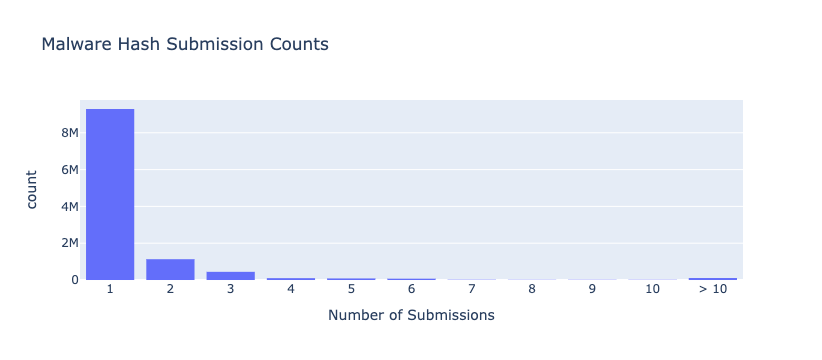
2. I lose the second field in the HIBP database, which is the number of times the password was found in the breach corpus.  This could be pretty useful if you consider that just finding a password once might be a different situation than finding it 30,000 times.  Again, my application doesn't need that info, and I was just throwing that data away anyway, so no problem there.

Sadly, the built-in disk save/load file format provided by pybloom is binary-only, and as far as I can tell, it's not guaranteed to be portable between machines of different architectures.  This isn't a problem for me at all, but I read in another of Troy Hunt's posts that hosting the download for 29GB files isn't cheap.  Perhaps with some extra work there'd be a portable way to serialize the Bloom filter, such that one could offer the much smaller populated filter instead, and anyone who just wanted to do simple existence checking at scale could use that.  

Still, I've showed that this kind of anonymous checking could be done, that it's efficient in terms of both storage and test speed, and quite easy to code.  Success!  

Hunting for Malware Critical Process Impersonation

A popular technique for hiding malware running on Windows systems is to give it a name that's confusingly similar to a legitimate Windows process, preferably one that is always present on all systems. The processes that Windows normally starts during boot (which I call the critical system processes) make good targets. Probably the most stereotypical example of this is malware running as scvhost.exe (a misspelling of the actual svchost.exe process). As it turns out, though, if you are collecting information about processes running on your systems, this type of activity is pretty easy to spot.

When it comes to comparing strings, most of us are familiar with equality since this is a basic operation in most languages. If str1 == str2 then they match! But string matching isn't always a binary answer. In this case, we specifically don't want to find strings that match exactly, nor do we want to find things that are wildly different. We're really looking for a narrow window of string similarity. That is, we're trying to identify processes that are so similar that they could easily be confused with the real thing, while not actually being identical to the real thing.

As it turns out, there are a number of ways to compute string similarity. They all work a bit differently and have particular strengths and weaknesses, but they typically accept two strings, compare them, and produce some sort of similarity score, like so:

score = compare(str1, str2)

As long as you're using the same algorithm for all the comparisons, you can use the scores to judge which pairs of strings are more or less similar than the others. Probably the most well-known algorithm for this is the Levenshtein distance. The resultant score is simply a count of the minimum number of single character insert, delete or modify operations it takes to convert str1 into str2. For example, the Levenshtein distance between 'svchost.exe' and 'scvhost.exe' (our example above) is 2 (delete the 'v', then add a new 'v' just after the 'c').

Because the algorithm is so simple, the Levenshtein distance would make a pretty decent choice for most uses, though in this case we're going to use a variant known as the Damerau-Levenshtein distance. The only difference here is that the Damerau-Levenshtein distance adds the transpose (switch adjacent characters) operation. Since transposition is one of the common techniques for creating confusingly similar filenames, it makes sense to account for this in our distance algorithm. With the Damerau-Levenshtein algorithm, the distance between 'svchost.exe' and 'scvhost.exe' is 1 (transpose the 'v' and the 'c').

With that background in mind, let's see how we can apply it across our network to detect malware masquerading as critical system processes.

The Hypothesis

Processes whose names are confusingly similar to those of critical system processes are likely to be malicious.

The Data

In my example, I'm looking at the full path to the binary on disk for any process that actually ran. Binaries that never ran will not be included in my analysis.  It's important to note that I'm comparing the path to the binary on disk, not the command line the system says was run, which is arguably the more inclusive check. In reality, you probably want to check both, since it's also quite common for malware to lie about it's command line. However, the command lines in my dataset require a lot of parsing and normalization, while the binary paths are pre-normalized. Using only the binaries makes a much clearer demonstration of the technique. Just be aware that for production use, you probably should spend the effort to normalize your command lines and check them, too.

One final note: on medium to large networks, you'll find that it won't be easy to hold all your process execution data in memory at once. My dataset is rather small, so I don't have to worry about it (again, it makes for a cleaner demonstration) but for larger-scale use, you may need to page your search results, convert the code into Spark or do something else clever to break things up a bit.

The Hunt

First, import some important modules.

import re

from ntpath import basename 

from jellyfish import damerau_levenshtein_distance

If you are a Python programmer, you probably recognize most of these.  The jellyfish module contains a number of routines that compute the "distance" between two strings, which is what this whole hunt is based on.

The following is a nested dictionary that defines the system processes we consider to be the most likely targets of this type of process impersonation. 

CRITICAL_PROCESSES = {'svchost.exe': {"threshold": 2,

                                      "whitelist":['c:\\windows\\system32\\sihost.exe',

                                             'c:\\windows\\microsoft.net\\framework64\\v4.0.30319\\smsvchost.exe']},

                      'smss.exe': {"threshold": 1,

                                   "whitelist":[]}, 

                      'wininit.exe':{"threshold":2,

                                     "whitelist":[]},

                      'taskhost.exe':{"threshold":2,

                                      "whitelist":['c:\\windows\\syswow64\\tasklist.exe',

                                             'c:\\windows\system32\\taskhostw.exe',

                                             'c:\\windows\\system32\\taskhostex.exe']},

                      'csrss.exe':{"threshold":1, 

                                   "whitelist":[]},

                      'services.exe':{"threshold":2,

                                      "whitelist":[]},

                      'lsass.exe':{"threshold":1,

                                   "whitelist":[]},

                      'lsm.exe':{"threshold":1,

                                 "whitelist":[]},

                      'winlogon.exe':{"threshold":2, 

                                      "whitelist":[]},

                      'explorer.exe':{"threshold":2,

                                      "whitelist":['c:\\program files (x86)\\internet explorer\\iexplore.exe',

                                             'c:\\program files\\internet explorer\\iexplore.exe']},

                      'iexplore.exe':{"threshold":2,

                                     "whitelist":['c:\\windows\\explorer.exe']}}

For each of these processes, we define a distance threshold (distances greater than zero but less than or equal to this value will be considered suspicious). We also keep a whitelist of the full path names to various legitimate binaries we found that would otherwise still register as suspicious. Feel free to tinker with these thresholds and whitelists, since they are likely to be very system dependent.  I had to run through several iterations with a subset of my data before I got values I was happy with.

The workhorse of this hunt is the similarity() function, which is defined as:

def similarity(proc, critical_procs=CRITICAL_PROCESSES):

    for crit_proc in critical_procs.keys():

        distance = damerau_levenshtein_distance(basename(proc).lower().decode('utf-8'), crit_proc.decode('utf-8'))

        if (distance > 0 and distance <= critical_procs[crit_proc]["threshold"]) and not proc in critical_procs[crit_proc]["whitelist"]:

            return (crit_proc, distance)

    return None

Pass similarity() the full path to a binary (e.g., c:\windows\system32\blah.exe) and the critical processes dictionary above, and it'll do the checks. If it finds something that's confusingly similar to one of the defined critical processes, it'll return a tuple containing the critical process to which it is similar and the distance score, like so: (crit_proc, distance). It'll stop checking the given process as soon as it finds a close match that's not whitelisted, so at most one result will be returned. If it finds no matches, it'll simply return None.

It's probably important to point out here that this function intentionally only compares the filenames and ignores the path.  In other words, it should find c:\windows\system32\scvhost.exe, but isn't concerned with things like c:\windows\temp\svchost.exe, where the filename is correct but the directory path is obviously bogus.  We can save this for a future hunt, though it's not hard to imagine combining the two!

At this point you need some process execution data!  The exact way you get this will vary from site to site, so I won't try to provide Python code for this.  Suffice it to say that my dataset is in a database, so I just queried the entire set via a SQL query:

SELECT process_guid, path FROM CarbonBlack WHERE type = 'ingress.event.procstart'

For each unique process execution, Carbon Black provides not only the full file path (the path value), but also a unique ID called the process_guid. If the process turns out to be suspicious, we'll need that so we can investigate further.  The code I used to pull this out of the database simply returns an list of tuples, like (process_guid, path), which is what I'll assume yours does, too.  If it comes some other way, the following code segment may need a bit of tweaking.

Finally, we just have to go through the results, weeding out the non-Windows processes (I have some Linux servers in my dataset) and compute similarity for each. If the similarity() function returns any results, the code prints them along with the GUID so we can follow up in our favorite threat hunting platform.

windows_regex = re.compile("^([a-z]:)|(\\SystemRoot)")

for i in processes_results:

    (guid, path) = i

    if windows_regex.match(path):

        res = similarity(path)

        if res:

            (crit_proc, distance) = res

            print "Process %s is suspiciously similar to %s (distance %d)" % (path, crit_proc, distance)

            print "\tGUID: %s" % guid

When it finds suspicious processes, the code will produce output similar to the following:

Process c:\windows\system32\csrrs.exe is suspiciously similar to csrss.exe (distance 1)

        GUID: 00000009-0000-0477-01d1-f282c48bc278

Process c:\program files\openssh\bin\ls.exe is suspiciously similar to lsm.exe (distance 1)
 GUID: 00000009-0000-0580-01d1-d883914e50c7
Process c:\program files\openssh\bin\ls.exe is suspiciously similar to lsm.exe (distance 1)
 GUID: 00000009-0000-057c-01d1-d87e79c39834
Process c:\program files\openssh\bin\ls.exe is suspiciously similar to lsm.exe (distance 1)
 GUID: 00000009-0000-1330-01d1-d87e72d3d61e
Process c:\program files\openssh\bin\ls.exe is suspiciously similar to lsm.exe (distance 1)
 GUID: 00000009-0000-13d4-01d1-d87d971196b0
Process c:\program files\openssh\bin\ls.exe is suspiciously similar to lsm.exe (distance 1)
 GUID: 00000009-0000-1268-01d1-d30d8b3d6765
Process c:\program files\openssh\bin\ls.exe is suspiciously similar to lsm.exe (distance 1)
 GUID: 00000009-0000-0254-01d1-d309333a60d1
Process c:\program files\openssh\bin\ls.exe is suspiciously similar to lsm.exe (distance 1)
 GUID: 00000009-0000-158c-01d1-d3091a4e674b
Process c:\program files\openssh\bin\ls.exe is suspiciously similar to lsm.exe (distance 1)
 GUID: 00000009-0000-1300-01d1-d3083db995cc

As you can see, we did find a few suspicious processes. One of them, csrrs.exe looks pretty suspicious! Fortunately, the rest were all the ls.exe binary provided as part of the OpenSSH package. Since OpenSSH is authorized on our network, this would be a good candidate to add to the lsm.exe whitelist so it doesn't keep coming up whenever we run our hunt.

Conclusions

Even though this hunt is looking at a very specific technique for hiding malware, it can still be effective.  If you have endpoint process execution data, looking for processes running with confusing names can be pretty helpful and fairly straightforward to implement.

Detecting Data Staging & Exfil Using the Producer-Consumer Ratio

In their FloCon 2014 presentation PCR - A New Flow Metric, Carter Bullard and John Gerth introduced the idea of the Producer-Consumer Ratio (PCR) for measuring and tracking shifts in the typical pattern of network communication for each host. PCR is calculated on a per-host basis, like this:

(bytes sent - bytes recvd)

-----------------------------

(bytes sent + bytes recvd)

This is an interesting metric, because it gives a good indication of the traffic pattern yet ignores many details that tend to complicate understanding, such as the actual volume of data sent or received, the number of flows, the amount of packets, etc. It boils everything down to one simple number in the range [-1.0,1.0]. They provided the following chart to give a rough idea how to interpret the PCR values:

PCR	host role
1.0	pure push - FTP upload, multicast, beaconing
0.4	70:30 export - Sending Email
0.0	Balanced Exchange - NTP, ARP probe
-0.5	3:1 import - HTTP Browsing
-1.0	pure pull - HTTP Download

The idea is that you can track the PCR for each host over time and look for shifts to identify significant changes that might indicate possible data exfiltration. I recently came across this technique as I was reviewing contributions to The ThreatHunting Project and though it sounded like a fun thing to play around with. I decided to give it a try on some test data I had laying around, just to see how it would work.

The Hypothesis

By comparing a host's baseline PCR to it's current PCR and looking for large shifts, we should be able to identify hosts that are exfiltrating the data to the Internet. By extension, we should also be able to use the PCR shift to identify central staging points for data, where threat actors gather it in preparation for exfiltration.

The Data

The data I used comes from a test lab which features a realistic corporate Windows environment in small scale (about 40 hosts) as well as a simulated user population that does things like access file servers, send/receive email, browse the web, etc. There's also a simulated Internet. 

In this lab, we monitor our network with Bro, so I used Bro's connection logs (conn.log files) as my data source. The exact format of these files doesn't really matter here, and you can easily adapt this to any flow data you happen to have (argus, SANCP, etc).

I should also point out that in this attack scenario, the same host was used for both data staging and data exfil. This isn't much of a problem when calculating PCR, since the staging and exfil detections each calculate PCR on a different subset of the data (those flows traversing the Internet perimeter for the exfil, and those staying only internal for the staging). Therefore, the combination of big inbound and outbound data transfers don't interfere with each other. Were I to ignore this and just compute PCR across all flows in the dataset, I'd probably have gotten a much more balanced PCR ratio, and therefore the staging and exfil on the same host would cancel each other out. This all just goes to show that PCR-based methods should always take the network vantage point(s) into account, or risk missing things that are anomalous in both directions.

Dealing With Production Datasets

Since this is a test lab, I have both a "clean" dataset (no threat actor activity) and one that contains a mixture of legitimate use and attack traffic (we'll call this the "dirty" dataset). Most readers, though, probably aren't so lucky. If you're trying to do this with your own data pulled from a production network, try defining the dirty data as everything during the previous 7 days and the clean data as anything before that (perhaps to a maximum of 30 or 60 days). Even though your "clean" data may not actually be totally clean, the more you have, the less likely any transient fluctuations are to distort your baseline PCRs.

Exfil Detection

Exfil is data going from inside our network to the Internet, so I started by filtering my flows to select only those where the source (orig_h) is an internal IP and the dest (resp_h) is an Internet host. In plain language, I selected only at flows that crossed the network's perimeter (transit to/from Internet).  Then I simply summed up the bytes sent and bytes received for each host (Bro's orig_ip_bytes and resp_ip_bytes columns, respectively).  

Note that since Bro records bi-directional flows, I had to calculate PCR for any host that appeared as either a source or a destination.  Further, each "destination" host not only received bytes, but sent some of its own, so I had to sum the resp_ip_bytes twice: once as the bytes received by the src host and once as the bytes sent by the dest host.  Ditto for the orig_ip_bytes, but in reverse.  In psuedo code, it would look something like this:

srchost_bytes_sent = sum(orig_ip_bytes)
srchost_bytes_recvd = sum(resp_ip_bytes)

dsthost_bytes_sent = sum(resp_ip_bytes)
dsthost_bytes_recvd = sum(orig_ip_bytes)

I was looking for hosts that have a fairly large PCR shift in the positive direction. In the extreme case, the baseline value would be -1.0 (a pure consumer) and the dirty value would be +1.0 (a pure producer). To make those hosts show up nicely, I calculated the shift as (dirty PCR - baseline PCR). In the best case, the shift would therefore be 2.0.

I constructed a scatter plot of PCR shift for each host, showing the baseline PCR on the X axis, the "dirty" PCR on the Y axis, and the amount of PCR shift as the color. The trend line provides an easy reference to see where "no PCR shift" would fall on the graph, and makes it a bit easier to eyeball the distances for the outliers.

Most hosts will tend to adhere closely to their own baselines, given enough data points. Therefore I would expect that the plot should look very much like a straight diagonal line (the graph of the line y=x). Furthermore, most colors should come out as a nice neutral grey.

Red hosts are more likely to be exfiltration, since those hosts shifted the most in a positive direction (towards being a producer). Theoretically, very blue hosts could indicate the exfil destinations (they suddenly consumed a lot more data than normal). However, being Internet hosts, we can't count on that. I only plotted hosts that have PCR values in both the baseline and in the "dirty" dataset. If I'd never seen a particular Internet host before (as is probably the case with threat actor infrastructure), it wouldn't show up. In practice, once you know the exfil host it's probably not too difficult to identify the host(s) that received the data, but if this were an issue you could try to do something smarter here.

As you can see in the graph above, the most red host isn't actually all that red (the exfil package wasn't very large), but it is the host that exfiltrated the data in our attack scenario.

Staging Detection

Data staging is defined as data moving purely internal to a network. This should show up as a hosts consumer ratio becoming more negative (the staging host). It may also show as some hosts (the hosts from which the data was stolen) becoming more positive if a lot of data was stolen from them.

For this part of the analysis, I specifically filtered the flows to only those  that both originated and terminated within the internal network.  As before, I calculated the PCR shift for each src & dest host in the dataset.  I calculated the PCR shift slightly differently here, since I was looking for different activity. In fact, I was trying to find the inverse of what I was looking for before, so I inverted the shift calculation, too. That is, in the best case, a system would go from a pure producer (PCR 1.0) to being a pure consumer (PCR -1.0). I calculated PCR shift here as (baseline PCR - dirty PCR), which would again mean a PCR shift of 2.0 for a host staging data.  I could have skipped this inversion, but it's an easy way to make the most significant shift look red on the graph, which I like.

I then constructed a new scatter plot of PCR shift for each host, showing the baseline PCR on the X axis, the "dirty" PCR on the Y axis, and the PCR shift as the color, just like the previous graph.

Again, hosts adhering to their own baselines would tend to fall near the diagonal y=x line, and be colored grey. Red hosts are more likely to be unusually large consumers of data relative to their own baselines, and therefore may represent systems being used as data staging points. In fact, as indicated above, the most red host is actually the host that was used to stage the stolen data. It's very red, indicating that it experienced a large shift.

Unlike in the previous graph, where blue points weren't likely to be very useful, they could very well indicate the sources of the stolen data in this graph. If the attacker stole a significant amount of data from any given system, it may be that the act of that victim host transferring it's data to the staging point caused a significant PCR shift in the producer direction. If so, those hosts would tend to fall out of the expected diagonal and be more blue than grey. In fact, most of the blue points here actually were the ones from which data was stolen. Most only lost a little data, it seems, though one host is quite blue, indicating that it may be the source of the bulk of the data.

Conclusions

Based on my test data, it seems like this has promise. In both cases, the "most red" point on the graphs corresponded to the data exfil or staging host. For staging, we were actually able to derive some additional information about the likely sources of the data that was stolen. We may not be able to rely on this in all cases, and it's likely to be much more complicated in a real enterprise environment, but where it's present, it may be quite useful. At least in my small dataset, tracking PCR shift proved an effective method for identifying both data staging and data exfiltration.